ssGSEA outputs
This page describes the single-sample gene set enrichment outputs generated by MTD Explorer.
ssGSEA summarizes host gene-set activity at the sample level. In MTD
Explorer, ssGSEA runs in comparison-capable analyses after the host expression
matrix has been converted to ssGSEA/host.gct.
Documentation example dataset
Figures shown on this page were generated from public Biomphalaria glabrata
RNA-seq data from NCBI BioProject
PRJNA1306560.
The example run contains infected, infection_failed, and uninfected
groups. Pairwise comparison examples use infected_vs_uninfected where
applicable. See Example dataset: Biomphalaria glabrata (PRJNA1306560) for the dataset origin, experimental groups, SRA accessions, and interpretation notes.
Current GMT selection behavior
The current default is:
This is different from the earlier legacy behavior in which the bundled MSigDB C2 symbols GMT was the default.
Available modes are:
| Value | Behavior |
|---|---|
auto |
Current default. Use the persistent eggNOG/GO master GMT created by Create_custom_host.sh for the selected host TaxID, intersect it with the current host.gct, and filter the resulting sets for this analysis |
default |
Explicitly use the bundled legacy MSigDB C2 symbols GMT |
FILE |
Use an existing user-provided GMT directly |
custom_eggnog is retained only as a deprecated backward-compatible alias and
is internally converted to auto.
Requirement for auto mode
The selected host reference must contain the persistent master GMT generated
by Create_custom_host.sh. If that file is missing, auto mode stops with
an error rather than silently falling back to MSigDB.
Analysis-specific GMT in auto mode
With auto, MTD Explorer does not rerun eggNOG annotation during every analysis.
It starts from the persistent host-reference master GMT and creates an
analysis-specific GMT after host.gct is available.
The generated files are stored under:
For host TaxID TAXID, the directory contains files such as:
custom_taxid_TAXID_eggNOG_GO.gmt
custom_taxid_TAXID_eggNOG_GO_analysis_summary.tsv
custom_taxid_TAXID_eggNOG_GO_analysis_set_table.tsv
The default filtering settings are:
| Filter | Current value |
|---|---|
| Minimum genes per retained set | 5 |
| Maximum genes per retained set | 500 |
| Minimum overlap genes | 100 |
| Minimum overlap percentage | 1 |
The analysis-specific GMT is the file actually supplied to ssGSEA in auto
mode. The methods table records the requested GMT setting, the resolved mode,
the persistent master GMT, and the analysis-specific GMT.
Main ssGSEA files
The core files are stored under:
Important files include:
host.gct is generated from the host TPM matrix and the samplesheet.
ssgsea-results-scores.gct contains the sample-level enrichment scores produced
by the ssGSEA implementation.
Original-feature plots
Plots using the original ssGSEA feature labels or GO IDs are stored in:
Typical outputs include:
ssGSEA/plots/ssGSEA_PCA_samples.png
ssGSEA/plots/ssGSEA_sample_correlation_heatmap.png
ssGSEA/plots/ssGSEA_top_variable_heatmap.png
ssGSEA/plots/ssGSEA_plot_summary.txt
Equivalent PDF versions may also be produced for supported plots.
GO-name-corrected plots
MTD Explorer also attempts to create a second set of plots with readable GO names. These are stored in:
The corrected score matrix and GO-resolution records include:
ssGSEA/ssgsea-results-scores_GO_names_corrected.gct
ssGSEA/go_term_resolution/ssGSEA_GO_ID_to_name_map.tsv
ssGSEA/go_term_resolution/quickgo_cache.tsv
The resolver first uses local information and supported correction mappings. By default, unresolved terms may also use the online QuickGO fallback and a secondary-ID/replacement search when internet access is available.
Typical corrected plots include:
ssGSEA/plots_GO_names/ssGSEA_PCA_samples.png
ssGSEA/plots_GO_names/ssGSEA_sample_correlation_heatmap.png
ssGSEA/plots_GO_names/ssGSEA_top_variable_heatmap.png
ssGSEA PCA
The PCA summarizes similarity among samples using the most variable ssGSEA features selected for the ordination.
Typical files are:
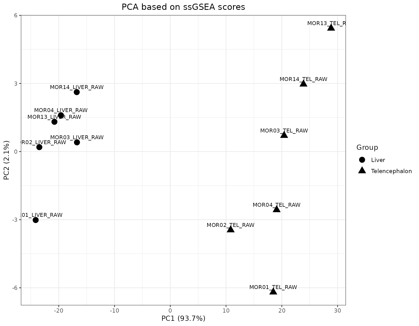
Samples that cluster near one another have more similar pathway/activity profiles. PCA is exploratory and should be interpreted together with the study design and differential score tables.
Sample correlation heatmap
Typical files are:
ssGSEA/plots/ssGSEA_sample_correlation_heatmap.png
ssGSEA/plots_GO_names/ssGSEA_sample_correlation_heatmap.png
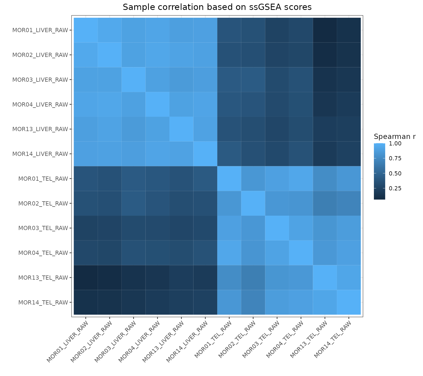
These heatmaps summarize sample-to-sample similarity across the ssGSEA score matrix.
Top-variable heatmap
Typical files are:
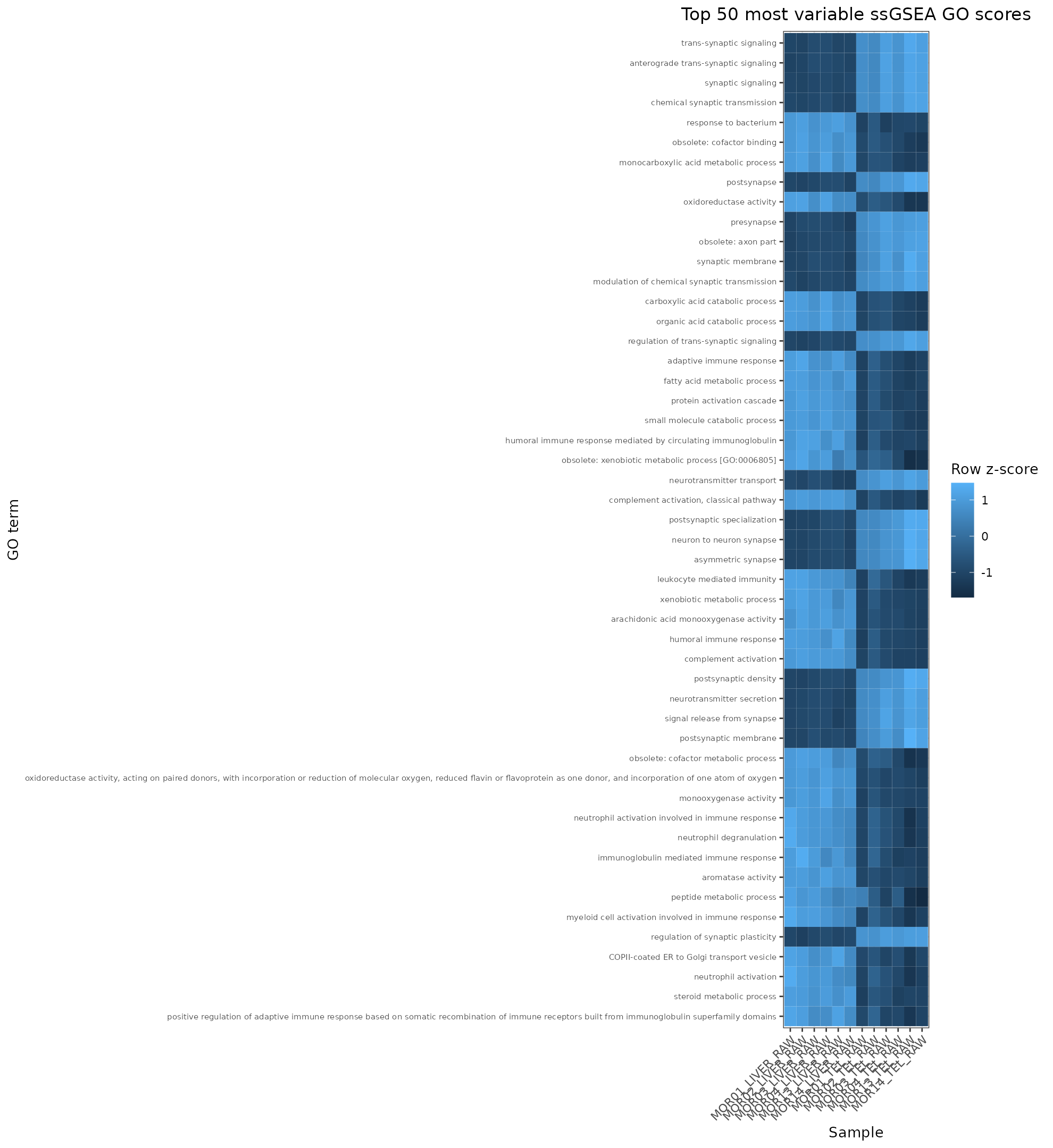
The plot highlights gene sets with the greatest variation across samples. It is useful for descriptive inspection but is not a substitute for formal group comparison.
Differential ssGSEA comparisons
Differential ssGSEA is now comparison-aware and supports studies with more than two groups.
When the samplesheet contains explicit group1 and group2 comparison columns,
those valid pairs are used. If no explicit comparison pairs are available, the
plotting workflow automatically generates all pairwise combinations among the
matched sample groups.
The comparison plan is written to:
and separately in the GO-name directory when the corrected plots are enabled.
The combined differential results are written to:
For multiple contrasts, each comparison also receives a numbered directory:
Each contrast can contain:
ssGSEA_differential_scores.tsv
ssGSEA_top_differential_boxplots.png
ssGSEA_top_differential_boxplots.pdf
The same structure is generated under plots_GO_names/ for the corrected GO
labels.
The differential table records the comparison index/name/source, group labels, sample counts, group means, the group1-minus-group2 difference, t-test and Wilcoxon p-values, and Benjamini-Hochberg-adjusted values. Multiple-testing adjustment is performed within each biological contrast across the tested terms.
When only one contrast exists, the workflow also preserves the convenient backward-compatible top-level differential boxplot in the plot directory.
Fewer than two groups
If fewer than two usable groups are available for the plotting step, formal ssGSEA differential testing is skipped rather than fabricating a contrast. A marker file is written:
This is a valid non-differential plotting outcome, not necessarily a pipeline error.
Top differential boxplots
For each valid contrast, the top differential boxplots visualize selected pathways/gene sets across the two groups.
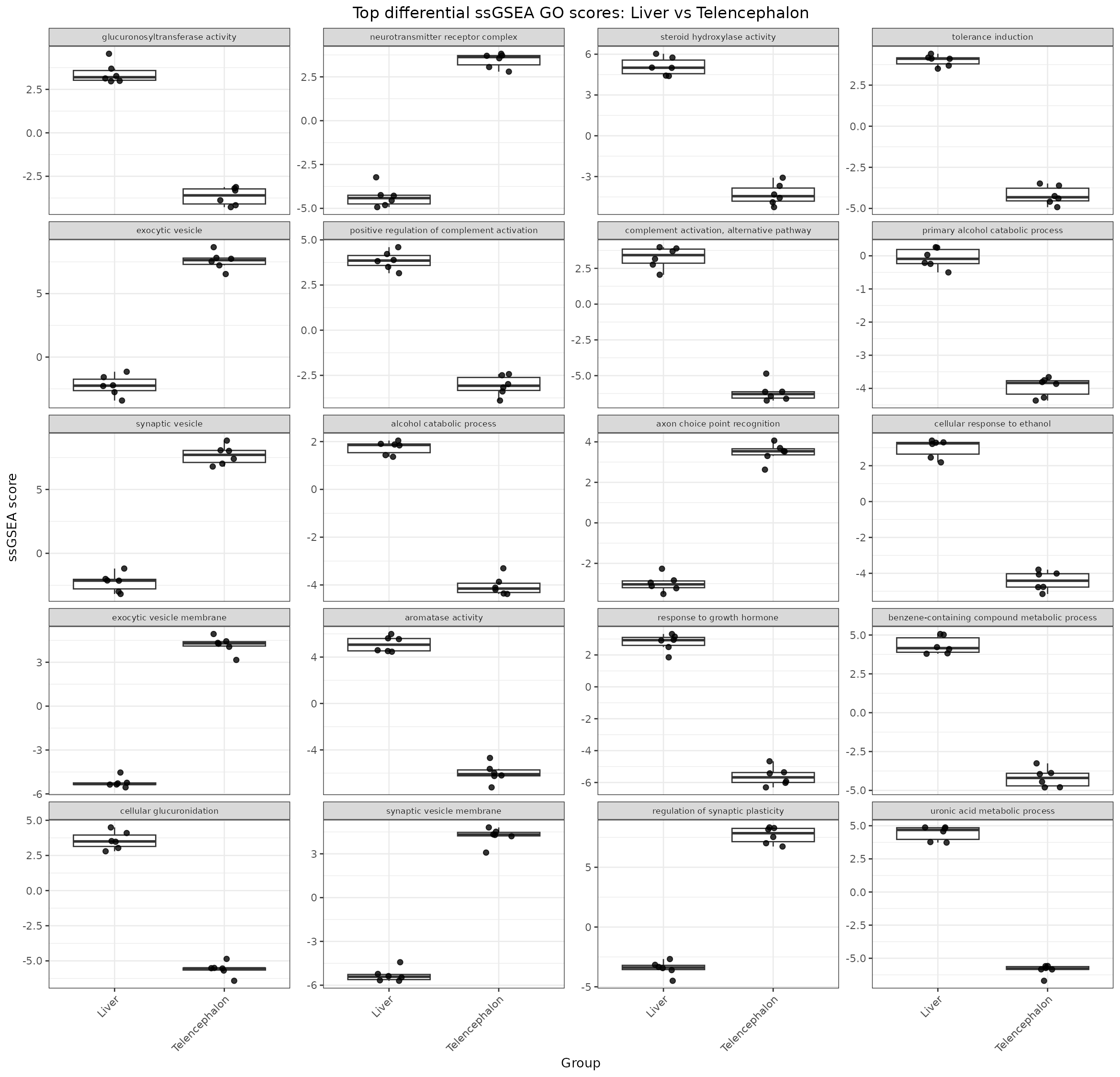
Use the corresponding ssGSEA_differential_scores.tsv table for statistical
interpretation rather than reading significance from the figure alone.
Recommended inspection order
For a current run, inspect:
ssGSEA/host.gct
ssGSEA/ssgsea-results-scores.gct
ssGSEA/custom_gmt_from_host_reference/ # when --ssgsea-gmt auto
ssGSEA/plots/ssGSEA_plot_summary.txt
ssGSEA/plots/ssGSEA_PCA_samples.png
ssGSEA/plots/ssGSEA_sample_correlation_heatmap.png
ssGSEA/plots/ssGSEA_top_variable_heatmap.png
ssGSEA/plots/ssGSEA_differential_comparisons.tsv
ssGSEA/plots/ssGSEA_differential_scores.tsv
ssGSEA/plots/differential/
ssGSEA/go_term_resolution/
ssGSEA/plots_GO_names/
methods/mtd_methods_run_parameters.csv
Not every item is present in every run. The custom GMT directory is specific to
auto, differential files require usable groups, and GO-name files depend on
the GO-name plotting step.
What these outputs can support
ssGSEA outputs can help assess whether host gene-set activity profiles cluster by sample or group, which pathways are most variable, and which pathway scores show statistical differences in defined biological contrasts.
What not to conclude
Do not interpret PCA separation or heatmap clustering as formal evidence of a group effect.
Do not assume the legacy MSigDB C2 GMT was used unless the run explicitly
requested --ssgsea-gmt default or the methods table confirms that mode.
Do not compare ssGSEA scores across runs without checking the GMT source, analysis-specific filtering, host reference, expression preprocessing, and samples included in each run.
When outputs may be missing
ssGSEA is skipped in exploratory/no-comparison pipeline runs. Individual plots or differential files may also be absent when there are too few samples, insufficient score variation, fewer than two usable groups, or no valid terms for a contrast.